5 + 3[1] 8Understand the definition of the following terms: script, object, and important R objects such as matrix, data.frame, and vector, statistical graph/chart, package, and function.
Understand the principal components of the RStudio interface and their roles.
Know how to generate a new RStudio project and access a previously created RStudio project.
Know how to create new folders within an RStudio project.
Know how to create, save, and open a script.
Know how to execute a line of code.
Understand how to install and load a package.
Understand how to load and visualize a dataset.
The RStudio interface is divided into four panes or quadrants. The specific layout may vary depending on user preferences, but a standard RStudio interface is as follows:
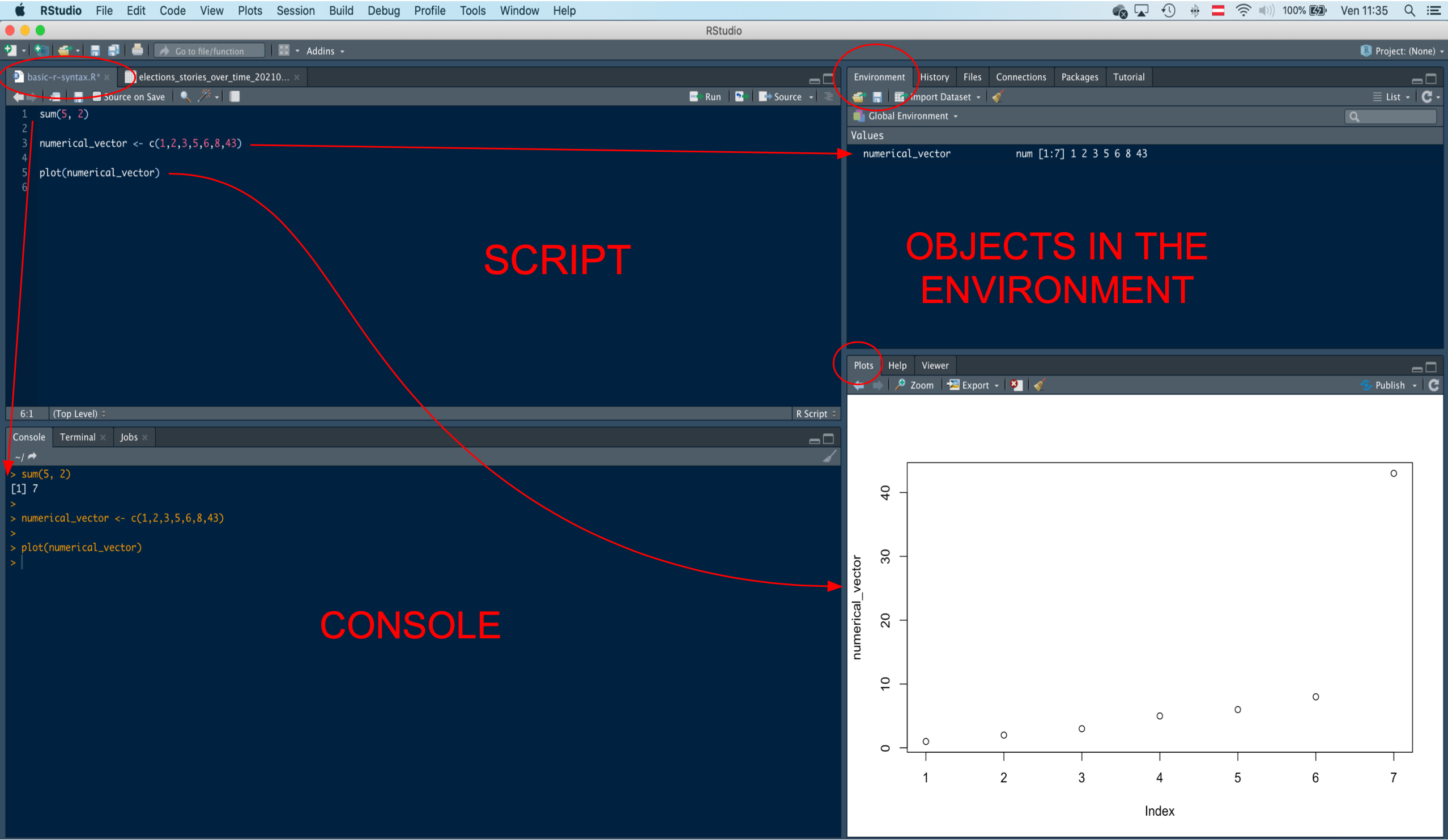
The top-left pane displays the scripts, which are text files containing a set of commands (code) used to perform analyses. Scripts are saved with the “.r” extension. The top-right quadrant includes the Environment window, where data sets and other objects created or loaded in a RStudio work session are stored. In R, objects refer to everything a user can manipulate, such as data sets, functions, and algorithms. This quadrant also contains tabs for Files, History, Connections, Packages, and more. The Files tab allows users to navigate files and folders to find scripts and data sets to upload.
The bottom-right quadrant is where graphical outputs, such as plots and statistical charts, are displayed. Statistical graphs or charts are visual representations of statistical data. This quadrant also contains a tab for R packages, which are collections of functions for performing specific operations and analyses. The Help section is also located here, providing information on functions and how to use them. Users can search for specific functions or type ?function_name in the console to access the Help section.
The bottom-left quadrant displays the R Console window, where code is executed and output is produced. Users can type and run commands directly in the console, but the code will not be saved unless it is written in a script.
When starting a new data analysis project, we create a dedicated work space. This dedicated work space is called a project. A project includes all the folders and files (e.g., scripts and data sets) necessary to conduct the analyses for the project’s purposes, as well as the outputs of the analysis (charts, tables, etc.).
To create a new project with RStudio, follows these steps:
ADA_MMCP (Advanced Data Analysis, Mediation Moderation Conditional Process Analysis).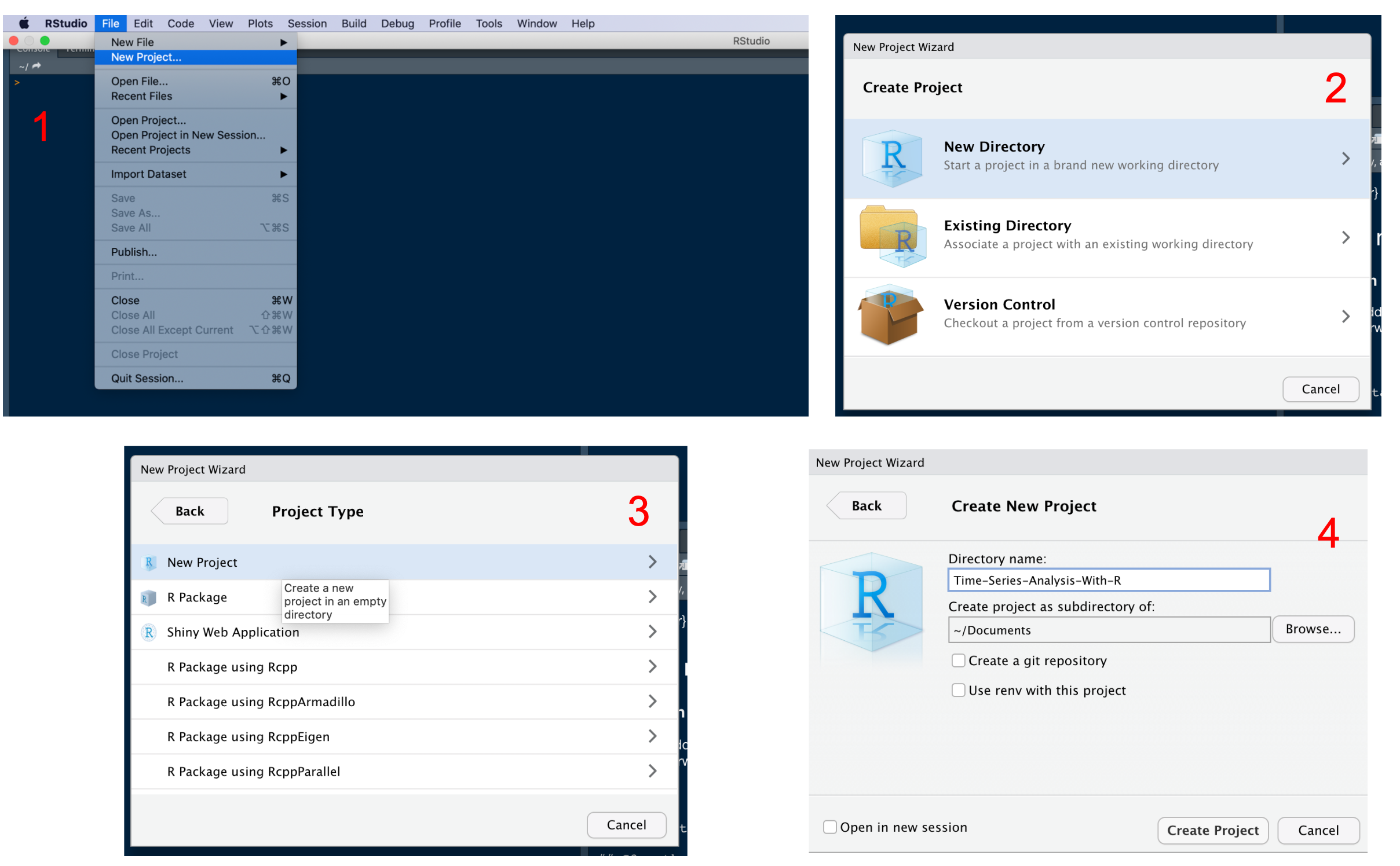
You have now created a project along with its own folder. The name of the folder is identical to that of the project. Inside the folder, there is a file with extension .Rproj and the same name of the project (e.g., ADA_MMCP.Rproj). This is the file you have to open whenever you want to work on the project.
Creating sub-folders within the main project folder can help organize the different types of files used in the project. For example, you may want to have a separate folder for data sets, another one for scripts, and another for outputs such as tables and graphs.
To create a sub-folder within the main project folder:
In the Files tab, navigate to the main project folder.
Click on the New Folder button.
Type the name of the sub-folder you want to create.
Press Enter.
Your new sub-folder will appear in the Files tab.

Now, create a folder for the data sets, called data. You will save here the data sets we are going to use during the course.
Once the project has been created, we can open a new script and save it. We said that a script is a file that contains code. Script files are automatically saved with extension .r. You can open, update, and save your script whenever you like. Saving code is important to save time! Otherwise, you would have to write the same code whenever you work on the project. Create a script named introduction_to_r. You will use it to write and run the code we are going to use in this learning unit.
To execute (or “run”) the code in the script, we can highlight the line of code we want to run, and then click the Run button. This button can be found on the top-right corner of the editor window. Alternatively, you can place the cursor on the row containing the code to be executed, and then click Run. Instead of the Run button, the code can be executed by using the Ctrl + Enter key combination (also Command + Enter on a Mac).
In your script introduction_to_r write a simple addition and execute it.
5 + 3[1] 8Now, save the script by clicking on the disk symbol you see in the top left corner of the editor. Close the script by clicking on the small “x” (upper right corner of the editor). Finally, in the “Files” window (upper left-hand quadrant), find the introduction_to_r script and reopen it in RStudio.
Packages (also libraries) are kinds of “toolboxes” containing sets of functions used to perform different types of operations.
R already includes several default functions and packages, but several additional packages are available. It is possible to install a package by using the menu (Tools/Install Packages…) or by using the function install.packages("name-of-the-package-here").
A very useful package is tidyverse. Tidyverse actually includes several other packages, such as ggplot2 to create charts, and dplyr to manipulate data sets (“data wrangling”).
install.packages("tidyverse")To use the functions contained in a package, you need to load the package into the work environment first. This can be done with by using the function library. For instance, we can load tidyverse with the following code:
library(tidyverse)── Attaching packages ─────────────────────────────────────── tidyverse 1.3.2 ──
✔ ggplot2 3.4.0 ✔ purrr 1.0.1
✔ tibble 3.1.8 ✔ dplyr 1.1.0
✔ tidyr 1.3.0 ✔ stringr 1.5.0
✔ readr 2.1.3 ✔ forcats 1.0.0
── Conflicts ────────────────────────────────────────── tidyverse_conflicts() ──
✖ dplyr::filter() masks stats::filter()
✖ dplyr::lag() masks stats::lag()There are a few important syntactic rules to keep in mind when writing code in R.
R recognizes lower and upper case letters. For example, the lowercase command sum is something completely different from the command Sum or SUM. In this case, while the function sum exists, there is no function called Sum or SUM.
# this works
sum(4, 6)

# this function does not exist (notice the error in the console)
Sum(4, 6)

# this function does not exist (notice the error in the console)
SUM(4, 6)
Only certain types of quotation marks are recognized by R. If you copy a command from the slides or other online sources, and paste them in R, you may encounter an error because of an incorrect character used for quotes.
# this is wrong (notice the error in the console)
glbwarm <- read.csv(file = data/glbwarm.csv)

# this is also wrong (notice the error in the console)
glbwarm <- read.csv(file = `data/glbwarm.csv`)

# this works
glbwarm <- read.csv(file = "data/glbwarm.csv")

# this also works
glbwarm <- read.csv(file = 'data/glbwarm.csv')You can load data into R in at least two different ways. First, you can navigate through your files/folders using the File window, and once you have found the data set, you can simply click on it and follow the RStudio semi-automated import process.
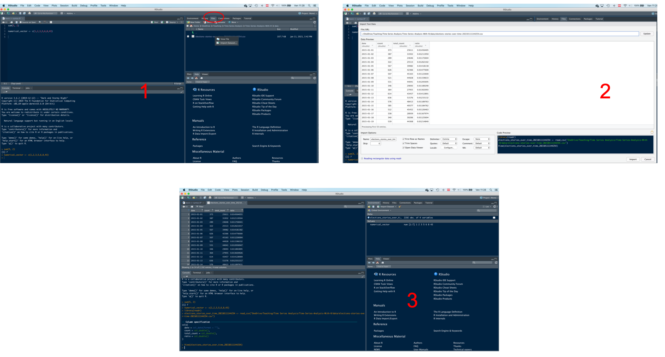
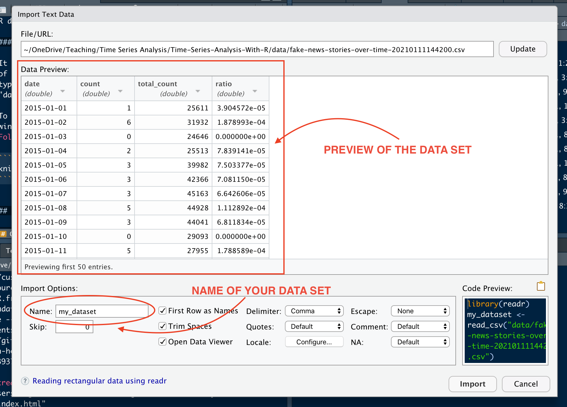
Otherwise, you can upload a data set by using a function. Since a data set can be saved in different formats (e.g., “.csv”, “.rds”, “.xlsx”, “.sav”, etc.), there are different functions to upload it. For instance, the function read.csv can be used to import a .csv file (one of the most common extension).
Download the data set “glbwarm.csv”, save it into your folder “data”, and load it in R by using the following code:
glbwarm <- read.csv(file = "data/glbwarm.csv")This function creates a object called glbwarm. You can see this object in the Environment window (top-right quadrant). We said that an object is something that can be manipulated in R. In this case, the object is a data set. You can manipulate it, for example, to perform analyses, create new data, etc.
Also note that, in R, we use an arrow <- to save the data set in an object. The arrow “transfers” the result of a function (its output) into an object. If you run a function without saving the output in an object through the arrow sign, the output is printed on the console.
read.csv(file = "data/glbwarm.csv") govact posemot negemot ideology age sex partyid
1 3.6 3.67 4.67 6 61 0 2
2 5.0 2.00 2.33 2 55 0 1
3 6.6 2.33 3.67 1 85 1 1
4 1.0 5.00 5.00 1 59 0 1
5 4.0 2.33 1.67 4 22 1 1
6 7.0 1.00 6.00 3 34 0 2This way you may take a look at the output (but this is not the right way to do that), but you cannot manipulate it. It is only when you create an object containing the output information of the function (using the arrow sign and a name for the object), that you can continue working on it.
To take a look at the data set, you can use the function head to print the first few rows in the console.
head(glbwarm) govact posemot negemot ideology age sex partyid
1 3.6 3.67 4.67 6 61 0 2
2 5.0 2.00 2.33 2 55 0 1
3 6.6 2.33 3.67 1 85 1 1
4 1.0 5.00 5.00 1 59 0 1
5 4.0 2.33 1.67 4 22 1 1
6 7.0 1.00 6.00 3 34 0 2You can also view the data set in a separate window by using the function View.
View(glbwarm)Another way to explore a data set is through the function str. This function allows the user to see the type of variables in the data set.
str(glbwarm)'data.frame': 815 obs. of 7 variables:
$ govact : num 3.6 5 6.6 1 4 7 6.8 5.6 6 2.6 ...
$ posemot : num 3.67 2 2.33 5 2.33 1 2.33 4 5 5 ...
$ negemot : num 4.67 2.33 3.67 5 1.67 6 4 5.33 6 2 ...
$ ideology: int 6 2 1 1 4 3 4 5 4 7 ...
$ age : int 61 55 85 59 22 34 47 65 50 60 ...
$ sex : int 0 0 1 0 1 0 1 1 1 1 ...
$ partyid : int 2 1 1 1 1 2 1 1 2 3 ...A similar function, included in the tidyverse package, is glimpse.
# load the package (load it just once in each R session)
library(tidyverse)
glimpse(glbwarm)
Rows: 815
Columns: 7
$ govact <dbl> 3.6, 5.0, 6.6, 1.0, 4.0, 7.0, 6.8, 5.6, 6.0, 2.6, 1.4, 5.6, 7…
$ posemot <dbl> 3.67, 2.00, 2.33, 5.00, 2.33, 1.00, 2.33, 4.00, 5.00, 5.00, 1…
$ negemot <dbl> 4.67, 2.33, 3.67, 5.00, 1.67, 6.00, 4.00, 5.33, 6.00, 2.00, 1…
$ ideology <int> 6, 2, 1, 1, 4, 3, 4, 5, 4, 7, 6, 4, 2, 4, 5, 2, 6, 4, 2, 4, 4…
$ age <int> 61, 55, 85, 59, 22, 34, 47, 65, 50, 60, 71, 60, 71, 59, 32, 3…
$ sex <int> 0, 0, 1, 0, 1, 0, 1, 1, 1, 1, 1, 0, 1, 0, 1, 1, 1, 0, 0, 0, 0…
$ partyid <int> 2, 1, 1, 1, 1, 2, 1, 1, 2, 3, 2, 1, 1, 1, 1, 1, 2, 3, 1, 3, 2…In this case, we can see that the first three variables are numerical (num), and the second three integers (int). Numeric (also double) is a data type that contains real numbers. Integers is a data type that contains integer numbers.
There are also other types of data, such as character (char) for character values, logical for logical values (TRUE and FALSE), and factors to describe items that can have a finite number of values (gender: male, female, other; education, etc.).
Sometimes, variables represents dates and times. Just to make an example of data set inclusing several type of data, we create a data set named data_set_example by running the following code.
glimpse(data_set_example)Rows: 4
Columns: 7
$ name <chr> "Karl", "Emma", "Sebastian", "Sarah"
$ gender <fct> M, F, Other, M
$ age <int> 30, 23, 12, 45
$ austrian <lgl> TRUE, FALSE, FALSE, TRUE
$ salary <fct> high, medium, low, medium
$ partisanship <dbl> -1.33, 4.56, -3.12, 2.54
$ date <date> 2020-01-01, 2020-03-01, 2020-01-02, 2020-01-03Data analysis operations basically consist of manipulations of objects through functions. An object is an entity composed of a name and a value (such as a number) or more complex information (such as a data set). The arrow <- sign is used to create objects, or to assign/update a value, if the object already exists.
Let’s make an example. Let’s create an object with name object_2 and value equal to 2.
object_2 <- 2Now, let’s write the name of the object in the script and run the command (put the cursor on the line of the name, and click run in the top right corner of the editor window, or Control + Enter). The value assigned to the object will be printed on the console.
object_2[1] 2Object names can be freely chosen. However, avoid using names that are already used for other objects and functions. For example, avoid giving the name read.csv to a data set, as this would overwrite the read.csv function. Similarly, if you use object_2 to save the output of another function, or to represent another value, you will delete the previous value (2):
object_2 <- 44
object_2
[1] 44object_2 <- 23 * 34
object_2[1] 782Sometimes you may want to delete an object from the environment. You can do that with the function rm (notice the object disappearing from the environment, in the Environment window).
rm(object_2)Since the object is equivalent to its value, an object with a numerical value can be used, for example, to perform arithmetical operations.
object_2 <- 2
object_2 * 10
[1] 20There are different types of object. We take into consideration some of the most important ones: Vectors, Matrices, Data Frames, Lists, Functions.
Vectors are sequences of values:
vector_of_numbers <- c(1,2,3,4,5,6,7,8,9,10)

vector_of_numbers
[1] 1 2 3 4 5 6 7 8 9 10A numeric vector can be used as a term for mathematical operations.
vector_of_numbers * 2 [1] 2 4 6 8 10 12 14 16 18 20vector_of_numbers + 3 [1] 4 5 6 7 8 9 10 11 12 13Vectors may consist of digits but also other symbols. For instance, a vector of letters is a character vector:
character_vector <- c("a", "b", "c")
character_vector
[1] "a" "b" "c"Another type of R object is the matrix (or array). A matrix is an object made up of a series of numeric vectors. In other words, it is a table where rows and columns contain numeric values.
a_matrix <- matrix(data = 1:50, nrow = 10, ncol = 5)
a_matrix
[,1] [,2] [,3] [,4] [,5]
[1,] 1 11 21 31 41
[2,] 2 12 22 32 42
[3,] 3 13 23 33 43
[4,] 4 14 24 34 44
[5,] 5 15 25 35 45
[6,] 6 16 26 36 46
[7,] 7 17 27 37 47
[8,] 8 18 28 38 48
[9,] 9 19 29 39 49
[10,] 10 20 30 40 50As matrices are mathematical objects, they can contain only numbers.
A data.frame is a very important object for data analysis and in this course we will work almost exclusively with data.frames.
Data frames are similar to matrices, but they can contain several types of data: numbers, characters (for instance, the texts of an answer), factors (such as gender, or ordered categories, such as “low”, “medium”, “high”), and dates. We have already encountered a couple of examples of data frames:
head(glbwarm) govact posemot negemot ideology age sex partyid
1 3.6 3.67 4.67 6 61 0 2
2 5.0 2.00 2.33 2 55 0 1
3 6.6 2.33 3.67 1 85 1 1
4 1.0 5.00 5.00 1 59 0 1
5 4.0 2.33 1.67 4 22 1 1
6 7.0 1.00 6.00 3 34 0 2head(data_set_example) name gender age austrian salary partisanship date
1 Karl M 30 TRUE high -1.33 2020-01-01
2 Emma F 23 FALSE medium 4.56 2020-03-01
3 Sebastian Other 12 FALSE low -3.12 2020-01-02
4 Sarah M 45 TRUE medium 2.54 2020-01-03Data frames are important because they represent data sets in R. For instance, if you import a csv or an Excel file in R, the corresponding R object is a data.frame. You can see the type of data by using the function class.
class(glbwarm)[1] "data.frame"class(data_set_example)[1] "data.frame"class(object_2)[1] "numeric"class(a_matrix)[1] "matrix" "array" The columns of a data set/data frame represent variables, and rows represent cases. For example, the global warming data set (glbwarm) comprises 815 rows/cases and 7 columns/variables. This data set results from measuring 815 persons on 7 dimensions (e.g., support for government, ideology, age, etc.).
head(glbwarm) govact posemot negemot ideology age sex partyid
1 3.6 3.67 4.67 6 61 0 2
2 5.0 2.00 2.33 2 55 0 1
3 6.6 2.33 3.67 1 85 1 1
4 1.0 5.00 5.00 1 59 0 1
5 4.0 2.33 1.67 4 22 1 1
6 7.0 1.00 6.00 3 34 0 2The function dim can be used to find the number of rows and columns of a data set. The first and second figure in the output is the number of rows and column, respectively.
dim(glbwarm)[1] 815 7The functions str or glimpse permits to see the names of the columns/variables. Another way to see them is using the function names.
names(glbwarm)[1] "govact" "posemot" "negemot" "ideology" "age" "sex" "partyid" We can access the columns of a data.frame by using the following syntax: name of the data frame, dollar sign $, name of the column. For instance, to access the column “age” of glbwarm:
glbwarm$age [1] 61 55 85 59 22 34 47 65 50 60You may have noticed that this is just a vector. Indeed, data.frames are object composed by a series of vectors.
Lists are another common type of object. Lists can be used to contain different types of objects. For example, a list may include a matrix, a number, and a data.frame. We will not work with this type of object in this course.
list(a_matrix, object_2, data_set_example)[[1]]
      [,1] [,2] [,3] [,4] [,5]
 [1,]    1   11   21   31   41
 [2,]    2   12   22   32   42
 [3,]    3   13   23   33   43
 [4,]    4   14   24   34   44
 [5,]    5   15   25   35   45
 [6,]    6   16   26   36   46
 [7,]    7   17   27   37   47
 [8,]    8   18   28   38   48
 [9,]    9   19   29   39   49
[10,]   10   20   30   40   50
[[2]]
[1] 2
[[3]]
       name gender age austrian salary partisanship       date
1      Karl      M  30     TRUE   high        -1.33 2020-01-01
2      Emma      F  23    FALSE medium         4.56 2020-03-01
3 Sebastian  Other  12    FALSE    low        -3.12 2020-01-02
4 Sarah M 45 TRUE medium 2.54 2020-01-03An object can also represent a function. We said that functions can be conceived as “mechanisms” that generate output from an input. Functions can transform other objects based on specific rules. For instance, addition is a function that receives two or more numbers as input and generates an output that corresponds to the sum of these numbers.
sum(1, 4)[1] 5A function has a name (the name of the function, like the name of any other object, e.g., the function sum) and one or more parameters. Arguments are written in parentheses, while the function name is left out of parentheses. Since functions transform objects, among the parameters there is always an object or a value, for instance a numerical value, which is the content the function is applied to. Usually, there are also several other arguments, either mandatory or optional, which modify the behavior of the function.
In this course we’ll use statistical function for performing linear regression in R, moderation, mediation, and conditional process analysis. For example, the name of the linear regression function in R is lm.
linear_model <- lm(glbwarm$govact ~ glbwarm$ideology)
summary(linear_model)
Call:
lm(formula = glbwarm$govact ~ glbwarm$ideology)

Residuals:
    Min      1Q  Median      3Q     Max
-4.7477 -0.7595  0.0287  0.8051  3.3109

Coefficients:
                 Estimate Std. Error t value Pr(>|t|)
(Intercept)       6.12419    0.12481   49.07   <2e-16 ***
glbwarm$ideology -0.37645    0.02867  -13.13   <2e-16 ***
---
Signif. codes:  0 '***' 0.001 '**' 0.01 '*' 0.05 '.' 0.1 ' ' 1

Residual standard error: 1.236 on 813 degrees of freedom
Multiple R-squared:  0.175, Adjusted R-squared:  0.174
F-statistic: 172.4 on 1 and 813 DF, p-value: < 2.2e-16Review the content of this lecture
Familiarize with R and RStudio
Detailed information on the R language (e.g., data structures, types of objects, etc.) can be found in the R Manual). A detailed overview of R programming language is beyond the objectives of this course, and not necessary to perform the analyses we’ll discuss. However, you can use this manual as a reference if you have doubts or would like to learn more.
Several resources about R are freely available online. YouTube features several good introductory videos to R. An important resource for programmers (both professionals and beginners) is https://stackoverflow.com.
Open the RStudio project you created in this learning unit
Open the script you created in this learning unit
Write and run a few mathematical operations in the script file (e.g., 3+2, 5/3, etc.)
Create a new object containing the output of the function sum (e.g., my_sum <- sum(4, 8)) and use this object to perform another mathematical operation of your choice
Save the updated script and close it
Create and save a new script
Copy all the data sets you find on Moodle in your “data” folder
Load one of the data set
Take a look at the data set using the functions View, str, and glimpse (remember to load the package tidyverse before using the glimpse function)
Access one of the column of the data set (name_of_dataframe + dollar sign $ + name of the column) using the dollar sign.